자전거 수요 예측
② Feature Engineering & 모델링
3. Feature Engineering
3-1. 이상치 제거
연속형 변수에 대해 boxplot을 그려 분포를 확인해보자
fig, axes = plt.subplots(6, 1, figsize = (12, 8))

sns.boxplot(data = train, x="temp", ax=axes[0])
sns.boxplot(data = train, x="humidity", ax=axes[1])
sns.boxplot(data = train, x="windspeed", ax=axes[2])
sns.boxplot(data = train, x="casual", ax=axes[3])
sns.boxplot(data = train, x="registered", ax=axes[4])
sns.boxplot(data = train, x="count", ax=axes[5])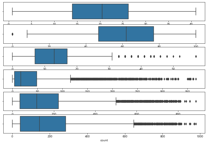
- windspeed, casual, registered, count에 이상치가 많이 존재하는 것을 확인할 수 있다.
이상치를 제거하고 다시 분포를 확인해보자
# 이상치 제거
cols = ['humidity', 'windspeed', 'casual', 'registered', 'count']
for col in cols:
    train = train[np.abs(train[col] - train[col].mean()) <= (3*train[col].std())]

fig, axes = plt.subplots(6, 1, figsize = (12, 8))

sns.boxplot(data = train, x="temp", ax=axes[0])
sns.boxplot(data = train, x="humidity", ax=axes[1])
sns.boxplot(data = train, x="windspeed", ax=axes[2])
sns.boxplot(data = train, x="casual", ax=axes[3])
sns.boxplot(data = train, x="registered", ax=axes[4])
sns.boxplot(data = train, x="count", ax=axes[5])

print(train.shape)  #(10886, 12) 변경 전
print(train.shape)  #(10212, 20) 변경 후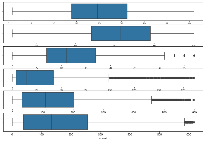
이상치가 잘 제거되었다
3-2. 정규화
count 값의 분포를 확인해보면 0에 몰려있다. 이에 로그를 씌워 정규화를 해주자
- 대부분의 기계학습은 종속변수가 정규분포를 갖는 것이 바람직함
# count 값의 데이터 분포 파악
figure, axes = plt.subplots(2, 2, figsize=(12, 10))

sns.distplot(train['count'], ax=axes[0][0])
stats.probplot(train['count'], dist='norm', fit=True, plot=axes[0][1])
sns.distplot(np.log(train['count']), ax=axes[1][0])
stats.probplot(np.log1p(train['count']), dist='norm', fit=True, plot=axes[1][1])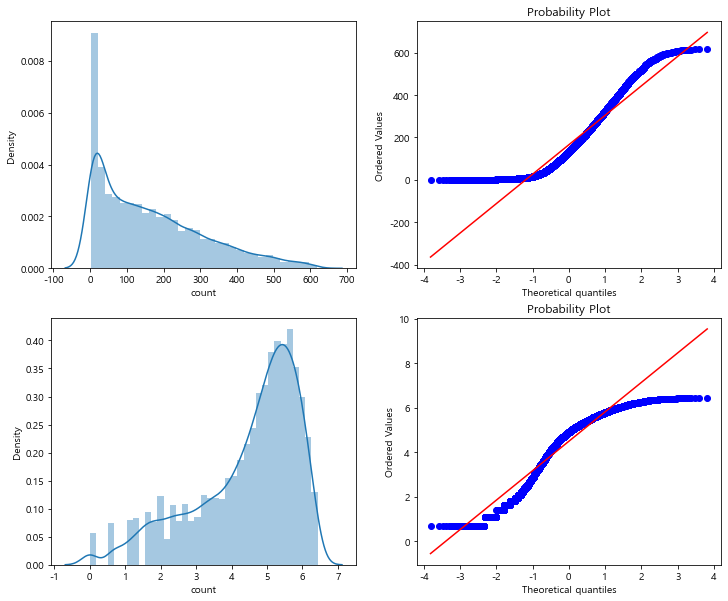
train['count_log'] = train['count'].map(lambda i:np.log(i) if i > 0 else 0)
train.head()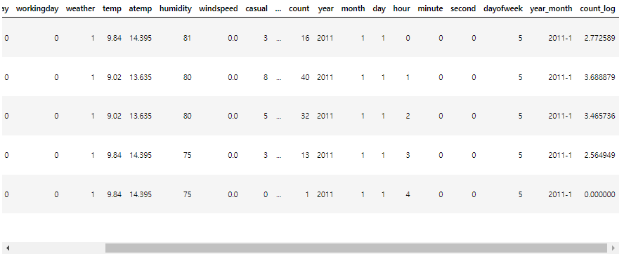
- log 씌운 값을 count_log 컬럼으로 생성해주었다.
3-3. 풍속이 0인 데이터 처리
EDA 과정에서 windspeed에 0인 값이 많이 존재하는 것을 확인했었다
train, test data에 대해 countplot으로 다시 한번 확인해보자
figure, axes = plt.subplots(2, 1, figsize=(12, 8))

plt.sca(axes[0])
plt.xticks(rotation=30, ha='right')
axes[0].set(title='train windspeed')
sns.countplot(data = train, x='windspeed', ax=axes[0])

plt.sca(axes[1])
plt.xticks(rotation=30, ha='right')
axes[1].set(title='test windspeed')
sns.countplot(data = test, x='windspeed', ax=axes[1])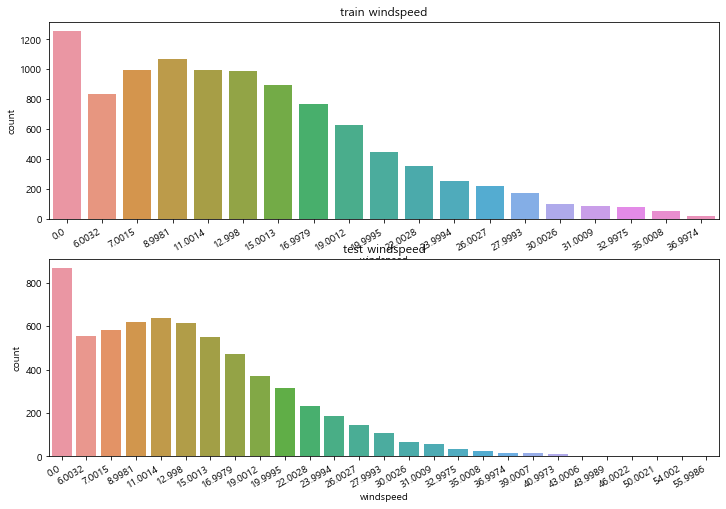
windspeed가 0인 값을 랜덤포레스트를 이용해 예측한 값으로 대체 할 것이다
train_wind0 = train.loc[train['windspeed'] == 0]
train_windnot0 = train.loc[train['windspeed'] != 0]
print(train_wind0.shape)  #(1256, 21)
print(train_windnot0.shape)  #(8956, 21)

# 함수 생성
def predict_windspeed(data):
    wind0 = data.loc[data['windspeed'] == 0]
    windnot0 = data.loc[data['windspeed'] != 0]

    # windspeed 예측할 피쳐 선택
    cols = ['season', 'weather', 'humidity', 'month', 'temp', 'year']

    windnot0['windspeed'] = windnot0['windspeed'].astype('str')

    model = RandomForestClassifier()
    model.fit(windnot0[cols], windnot0['windspeed'])

    pred_wind0 = model.predict(X = wind0[cols])
    wind0['windspeed'] = pred_wind0

    data = windnot0.append(wind0)
    data['windspeed'] = data['windspeed'].astype('float')

    data.reset_index(inplace=True)
    data.drop('index', inplace=True, axis=1)

    return data

# train, test data 변경
train = predict_windspeed(train)
test = predict_windspeed(test)
train[train['windspeed'] == 0]
figure, axes = plt.subplots(2, 1, figsize=(12, 8))
plt.sca(axes[0])
plt.xticks(rotation=30, ha='right')
axes[0].set(title='train windspeed')
sns.countplot(data = train, x='windspeed', ax=axes[0])
plt.sca(axes[1])
plt.xticks(rotation=30, ha='right')
axes[1].set(title='test windspeed')
sns.countplot(data = test, x='windspeed', ax=axes[1])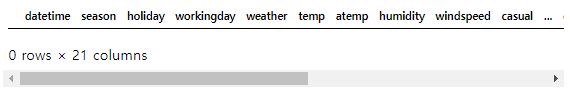
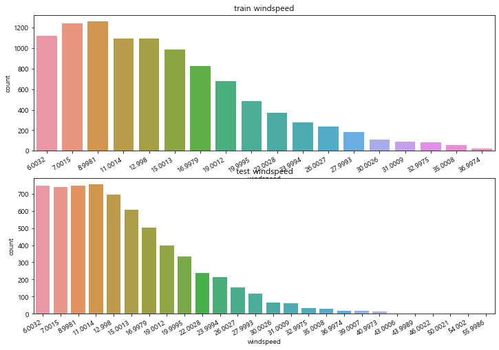
- windspeed가 0인 값이 사라진 것이 확인된다
3-4. 범주형 변수 변경
범주형인 변수들을 category 형태로 바꿔주자
cols = ['season', 'holiday', 'workingday', 'weather', 'dayofweek', 'month', 'hour', 'year']

for col in cols:
    train[col] = train[col].astype('category')
    test[col] = test[col].astype('category')

train.info()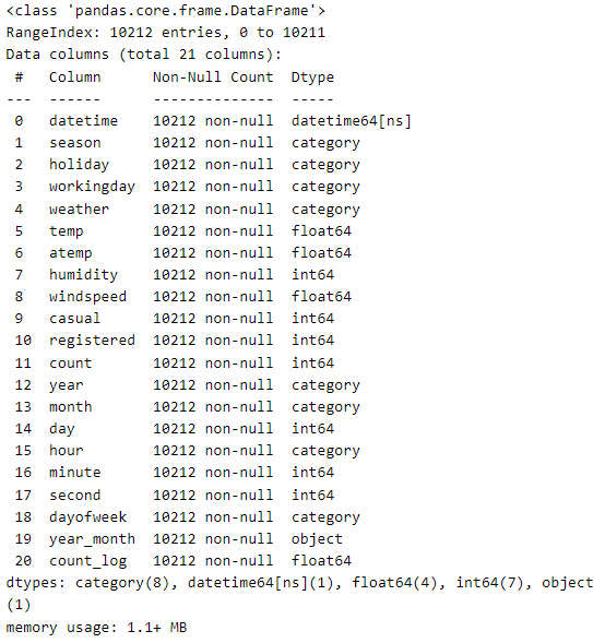
4. 모델링
4-1. 변수 선택
먼저 피쳐로 사용할 변수를 리스트로 만들어준 뒤 train_input, train_target, test_input을 만들어주자
target으로는 'count'가 아닌 위에서 만들었던 'count_log'를 사용할 것이다
features = ['season', 'holiday', 'weather', 'temp', 'humidity',
           'windspeed', 'year', 'month', 'hour', 'dayofweek']

train_input = train[features]
print(train_input.shape)
train_input.head()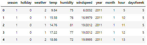
test_input = test[features]
print(test_input.shape)
test_input.head()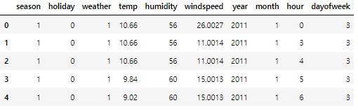
label_name = 'count_log'

train_target = train[label_name]
print(train_target.shape)
train_target.head()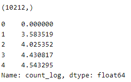
4-2. RMSLE & 모델 학습
- 자전거의 일별 대여량을 예측하는 문제이므로 회귀(Regression) 모델을 사용할 것이다
- 이 대회는 회귀 평가 지표중 하나인 RMSLE(Root Mean Squared Logarithmic Error) Score 로 평가
먼저, RMSLE 함수를 만들어주자 ( 0에 가까울수록 좋음 )

# RMSLE 함수
def RMSLE(predicted_values, actual_values):

    predicted_values = np.array(predicted_values)
    actual_values = np.array(actual_values)

    log_predict = np.log(predicted_values + 1)
    log_actual = np.log(actual_values + 1)

    difference = log_predict - log_actual
    difference = np.square(difference)

    mean_difference = difference.mean()
    score = np.sqrt(mean_difference)

    return score

rmsle_score = make_scorer(RMSLE)
kfold 교차 검증과 GradientBoostingRegressor 모델로 학습을 진행할 것이다
# KFold
kfold = KFold(n_splits=10, random_state=42, shuffle=True)

from sklearn.ensemble import GradientBoostingRegressor
model = GradientBoostingRegressor(random_state=42)
scores = cross_validate(model, train_input, train_target,
                       return_train_score=True, n_jobs=-1)

# train, val data 점수
print(np.mean(scores['train_score']), np.mean(scores['test_score']))
# 0.9194017180370215 0.9018757705894085


# RMSLE 점수
score = cross_val_score(model, train_input, train_target, cv=kfold, scoring=rmsle_score)
score = score.mean()
score  #0.13077674772551076

model.fit(train_input, train_target)- train, val data 점수를 보면 과대/과소적합 없이 괜찮은 성능을 내는 것으로 보인다
- RMSLE 점수를 확인해도 0.13으로 좋은 점수라는 생각이 든다
4-3. 예측 및 제출
이제 test_input에 대해 예측을 해준 뒤 submission 데이터를 만든뒤 제출하면 된다
pred = model.predict(test_input)
submission = pd.read_csv("C:/data/Bike/sampleSubmission.csv")
submission['count_log'] = pred

# count_log를 다시 count로 바꾸기
submission['count'] = np.exp(submission['count_log'])
submission.drop('count_log', axis=1, inplace=True)
submission.head()

submission.to_csv("C:/data/Bike/bike_submission.csv", index=False)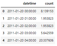
결론
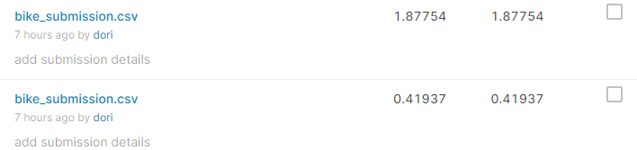
점수가 이상하다...!
이 과정대로 캐글에 제출하면 Score가 1.854로 나온다
FE에서 어느 부분을 제외한 뒤 제출했을 때는 0.419가 나왔었는데 위 코드에서 어디가 점수를 낮춘건지 아직 찾지 못 했다..
4-2에서 점수는 괜찮게 나오는데 제출하면 점수가 왜 내려가는지 잘 모르겠다 ㅠㅠ
다시 보고 찾아내면 글도 수정할 예정이다!
'Python > 데이터분석 실습' 카테고리의 다른 글
| [Kaggle] Titanic 생존자 예측 ② Feature Engineering & 모델링 (0) | 2022.05.11 |
|---|---|
| [Kaggle] Titanic 생존자 예측 ① 데이터 확인 & EDA (0) | 2022.05.09 |
| [Kaggle] 자전거 수요 예측 ① 데이터 확인 & EDA (0) | 2022.05.03 |
| [Kaggle ] Pima Indians Diabetes 예측 ② 데이터 전처리 후 모델 학습/예측 (0) | 2022.03.01 |
| [Kaggle] Pima Indians Diabetes 예측 ① EDA, 시각화 탐색 (0) | 2022.02.28 |